pst-plot -- Math function examples

| Main page |
|
Index |
| Bug list |
| Documentation |
| Doc errors |
| Examples |
| 2D Gallery |
| 3D Gallery |
|
Packages
|
|
References
|
|
CTAN Search CTAN: Germany USA |
|
Statistics |
|
Extended translation of the the 5th edition |
|
the 7th edition, total of 960 colored pages |
|
2nd edition, 212 pages, includes 32 color pages |
|
 |
|
 |
|
 |
|
 |
|
 |
|
|
|
|
|
 |
|
 |
arccos(x) | Axes |
Bessel curves |
Chirikov function | Clipping math functions | Cubic root |
Differential equations | Discontinued plots |
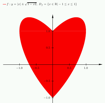
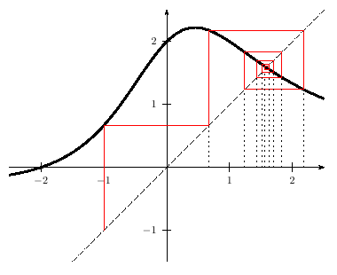
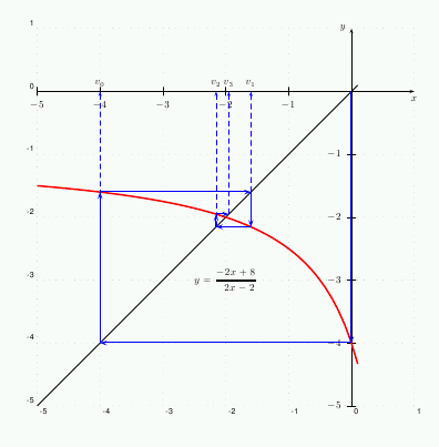
filling areas between two curves | Fixpoint |
Gaußcurve | Grid -- redefinition | Gridstyle |
Hyperbola |
Integer function | Interrupted x-axis | Introduction | Iterated curves |
Label position | Label step | Lissajous figure | ln(x) | Logarithmic axes |
Maxwell-Boltzmann velocity probability | Multiple axes |
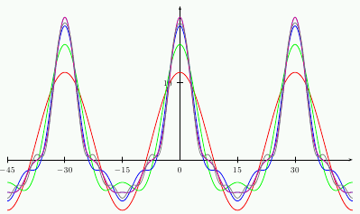
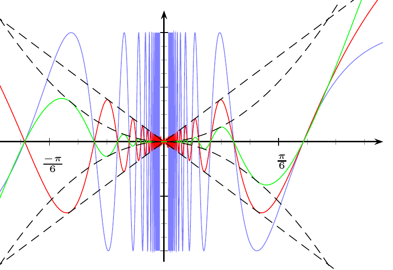
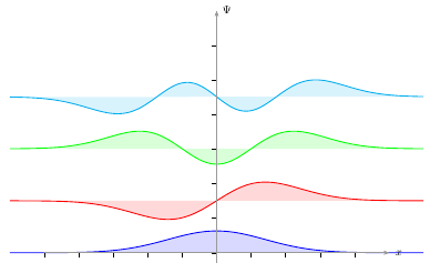
Oscillator function | Quantum harmonics oscillator |
Parabola | Parametric plots | Plot of arccos(x) | Plot of arctan(x) | Plot of sin(1/x) | Plot of sin(x)/x) | Polynomial function | PostScript procedures | Printing function values |
Quantum harmonics oscillator |
Random noise | Reciprocal function | Riemann function | Root sqrt[3]{x} | RPN-Expression converter |
Save calculated points in a file | Simple Examples | sin(1/x) | sin(x)/x) | sin function with a random noise | shaded areas under a curve | Special coordinates | Step function (Riemann) |
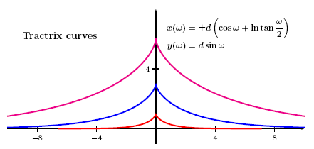
tan(x) | Tractrix curve | Trigonometric labels |
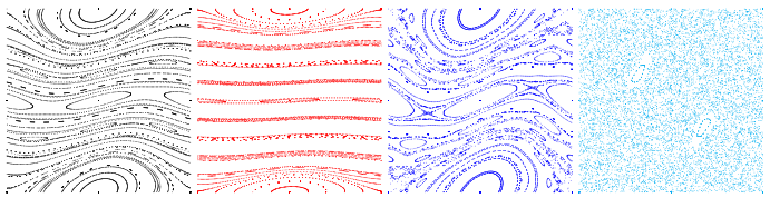
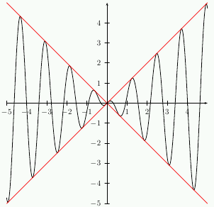
| Chirikov function |
|---|
 |


|
 |
|
|
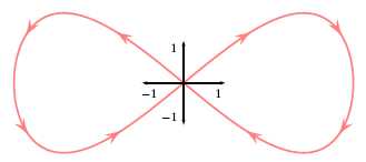
| Lissajous figure | |
|---|---|
 |
 |
|
|
|
| Iterated curves | Fun :-) |
|---|---|
 |
 |
|
|
|
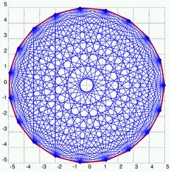
Sometimes it may be useful to save every single (x|y) data record of an external file as a node
to draw lines or something else from point to point. The following example first saves all
points (plotpoints=20) of a circle in an external file data.ps. This is done by
PostScript(!), this is the reason why you have to run the PS-output once with ghostscript to
build this file. In a second run the document reads the data file, saves all data records as
nodes N<#>, plots it with the fileplot
macro. After that all nodes are just for fun connected by a line with each other.The files needs the package pstricks-add for the modulo function to draw all this lines:
\multido{\iA=1+1}{\plotpoints}{\psdot(N\iA)%
  \multido{\iB=\iA+1}{\plotpoints}{%
    \modulo{\iB}{\plotpoints}\nextPoint%
    \psline[linewidth=0.1pt,linecolor=blue]%
	   (N\iA)(N\nextPoint)%
  }%
}%
| ||
|

|
|
|
|
|
| Oscillator function | |
|---|---|
 |
 |
|
|
|
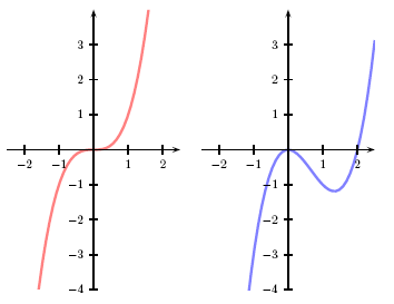
| Polynomial | |
|---|---|
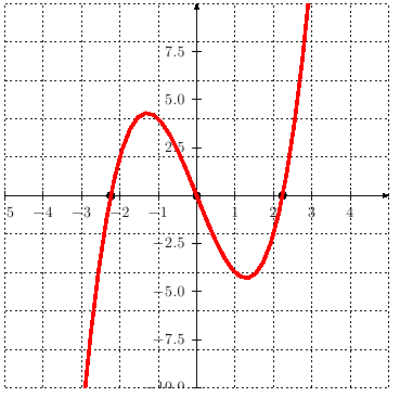 (The zeros are calculated and marked by the macro) |
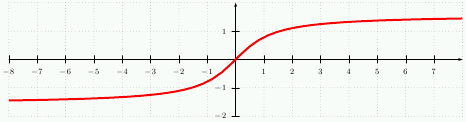
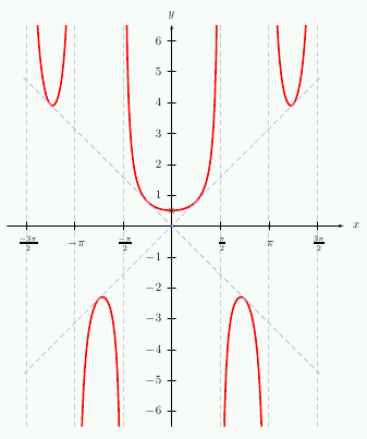
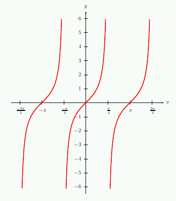
The inverse function of tan(x), the atan(x), has the syntax
y=atan(nominator/demoninator) and the values are in the range of 0..360°.
This is in difference to the default definition of -90...+90°. The following example
shows a plot which uses this last definition (needs pstricks-add).
For the plot of a tan(x) go here
It is also possibe to get the same result with the \parametricplot macro, which
is shown in the above source file and pdf.
|
|
|
|
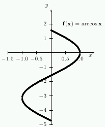
acrcos x |
Reciprocal function |
|---|---|
 |
 |
|
|
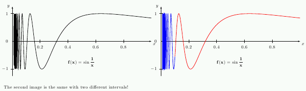
| sin(x)/x | Special coordinates |
|---|---|
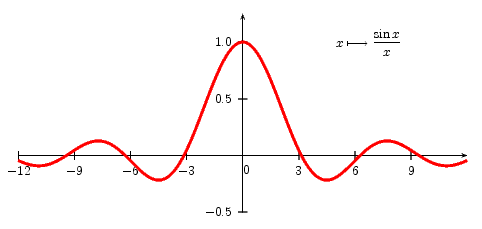
|  |
|
|
|
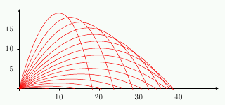
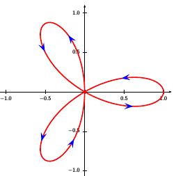
| Parametric plots | ||
|---|---|---|
 |
 |
 |
|
|
|
|
 |
 |
|
|
|
|
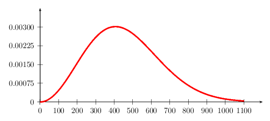
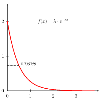
| Maxwell-Boltzmann | |
|---|---|
|
The file enclosed below plots the Maxwell-Boltzmann velocity probability
distribution for a sample of gas at 300 K and molar mass 40 g/mol.
|
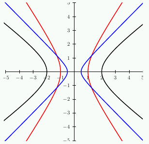
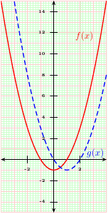
| Parabola | Hyperbola |
|---|---|
 |
 |
|
|
|
|
 |
|
|
|
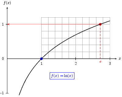
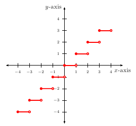
| Natural logarithm | Integer function |
|---|---|
 |
 |
|
|
|
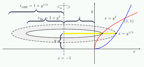
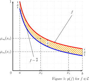
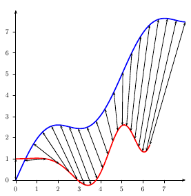
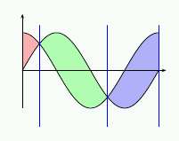
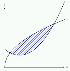
| Shaded areas between curves | ||
|---|---|---|
 |
 |
 |
|
|
|
|
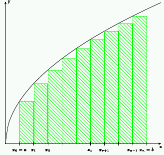
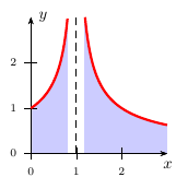
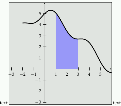
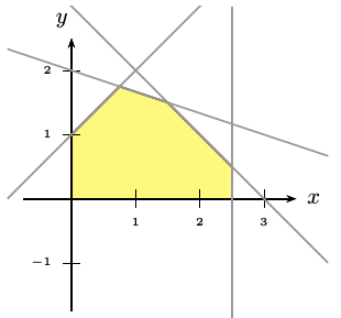
| Shaded areas under a curve | |
|---|---|
 |
 |
|
|
|
| Printing function values | |
|---|---|
 |
 |
|
|
|
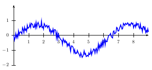
| Clipping math functions | sin with a random noise | Special Grid |
|---|---|---|
| Plotting math functions with pst-plot is given by the range xMin<x>xMax. When there are y values out of the by pspicture defined area, then it is easier to clip the plotting area instead of guessing the minimal and maximal useful x value. The example shows different possibilities to clip the plotting area. | ||
 |
 |
 |
|
|
|
|
 |
||
|
|
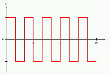
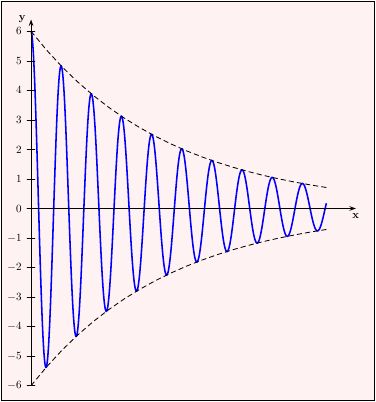
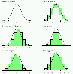
| Step functions | Quantum harmonics oscillator |
|---|---|
 |
 |
|
|
|
| Fixpoint | |
|---|---|
There is also a macro \psFixpoint in the package pst-plot which allows
easier solution than these two ones which work with \multuido.
|
|
 |
 |
|
|
|
| Discontinued plots with yMaxValue option | |
|---|---|
 |
 |
|
|
|
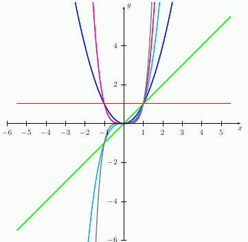
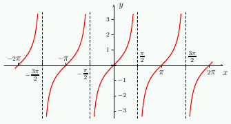
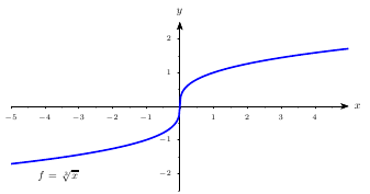
| Tangens with pst-plot | Cubic root |
|---|---|
 |
 |
|
|
|